Acknowledge
The chlorophyll-a data is modified from:
Adams, H. (2021) Rates and timing of chlorophyll-a increases and related environmental variables in global temperate and cold-temperate lakes. Federated Research Data Repository. https://doi.org/10.20383/102.0488
The climate data for NA lakes is synthesized from:
Wang, T., Hamann, A., Spittlehouse, D. L., & Carroll, C. (2016). Locally downscaled and spatially customizable climate data for historical and future periods for North America. PloS One, 11(6), e0156720. https://doi.org/10.1371/journal.pone.0156720
Note: The software version used in this study uses different historical data than the official release available at http://climatena.ca.
The climate data for EU lakes is synthesized from:
Marchi, M., Castellanos-Acuna, D., Hamann, A., Wang, T., Ray, D., & Menzel, A. (2020). ClimateEU, scale-free climate normals, historical time series, and future projections for Europe. Scientific Data, 7, 428. https://doi.org/10.1038/s41597-020-00763-0
Data Collection:
The chlorophyll-a data was divided by two parts, lakes in North America and Europe by using Excel and .csv format. The "=VLOOKUP()" function is used to pair the lake names with country. Due to lack of climate data, the samples in China and Japan are delected.
sample numbers is calculatd by using "=SUMIF()" function.
growth_window_length, chla_rate, max_chla and acc_chla are calculated by using "=AVERAGEIF()" function.
Values for all lakes are averaged or sumed (eg. sample size) except for some representative numbers such as climate zone number.
Then the data was divided into two documents, NA and EU. The format of documents are csv.
Location: Windermere North Basin was chosen to plot the time vs climate factors and algae growth line graphs.
Then ClimateEU software was used for the Europe climate data; Climate NA software is used for North America climate data.
After this, all the datasets are combined in one csv. file.
Then, Rstudio is used for remaining data analysis.
The version of Rstudio: RStudio 2022.12.0+353 "Elsbeth Geranium" Release (7d165dcfc1b6d300eb247738db2c7076234f6ef0, 2022-12-03) for Windows
Mozilla/5.0 (Windows NT 10.0; Win64; x64) AppleWebKit/537.36 (KHTML, like Gecko) RStudio/2022.12.0+353 Chrome/102.0.5005.167 Electron/19.1.3 Safari/537.36
The Google Earth Pro is used to plot all the locations on the map.
The version of Google Earth Pro: 7.3.6.9345 (64-bit)
Locations:
The choice of high-latitude regions in North America and Europe for the study on algae and climate variables may be due to their unique climates, especially relatively low temperatures, which can impact local algae species. These regions also offer a diverse array of algae species, making them ideal for studying algae diversity and how different species compositions respond to changes in climate variables. Also, these regions have relatively well-established research infrastructures and monitoring programs that collect data on climate variables, making it easier to obtain necessary data for study and compare results across locations.
Map 1: The location for lake samples in both EU and NA. Most lakes in the dataset are located at high latitude which are between 50 and 60° N. There are 352 samples in total. (Google Earth Pro)
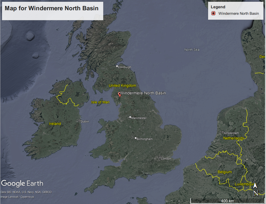
Map 1: The location for Windermere North Basin, United Kingdom. (Google Earth Pro)
Data Analysis
- Bar plot was used to count the number of samples under different tropic status.
- Correlation and the graph were used to see the relationship between two variables.
- Principle component analysis (PCA) graph was plotted and the vectors were used to see the relationships between variables.
- Boxplots and ggplot graphs were used to see the difference between lake under different trophic status.
- ggparis shows the distribution and difference of samples through matrix.
- Linear regression (lm) was used to plot the trendlines.
- Nonmetric multidimensional scaling (NMDS) was used to explore and visualize potential differences or similarities between groups.
- The direct gradient analysis with NMDS was used to test relationships between response variables, predictor variables and regions (EU, NA).
- For PCA, NMDS and direct gradient analysis with NMDS, euclidean distance was used as the variables in this study are continuous.
- Line graphs were used to see the delayed effect by climate change.
