The Figure 1 presents overall data on the trophic status of 354 lakes. As indicated by the graph, 20 of the lakes are oligotrophic, 67 are mesotrophic, 242 are eutrophic, and 24 are hypereutrophic. The eutrophic is the domain trophic status of the lake at high latitude. This figure shows that Eutrophic was the dominant trophic status domain observed in lakes located at high latitudes.
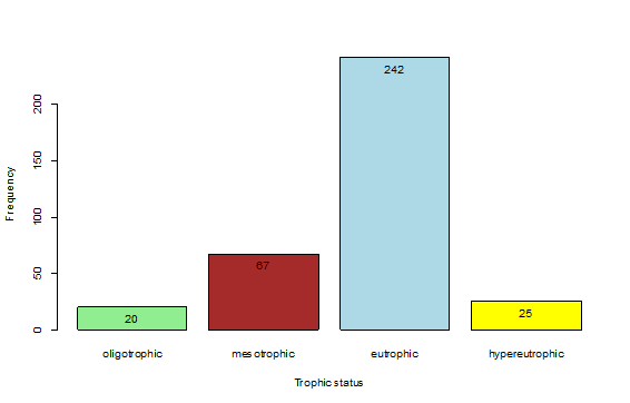
Figure 1: Bar plot which shows the number of lakes in each trophic status category. There are 354 samples in total.
R script
The Figure 2a and 2b present overall data on the trophic status in North America and Europe. There are 101 samples in Figure 2a and 253 samples in Figure 2b. In both Figures, the eutrophic is the dominant trophic status at high latitude lakes in both North America and Europe.
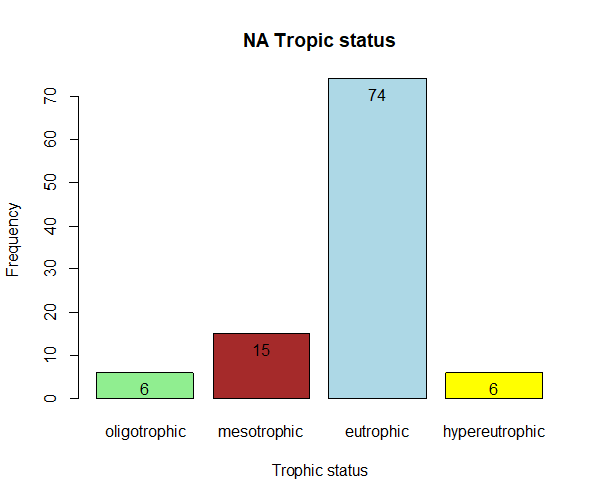
Figure 2a. Bar plot which shows the number of lakes in each trophic status category in North America. There are 101 samples in total.
|
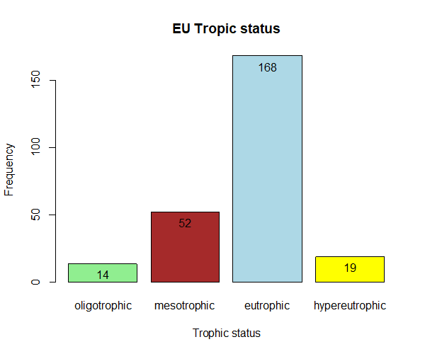
Figure 2b. Bar plot which shows the number of lakes in each trophic status category in Europe. There are 253 samples in total
|
The Figure 3a and 3b below shows the relationships between trophic state index in North America and Europe. The trendline was plotted by using y=ax^2+bx+c. Through the tredlines, we can see that as TSI increases, the growth rate of chlorophyll-a in lakes also increases. We can also observe that the increase in Europe is greater than in North America.
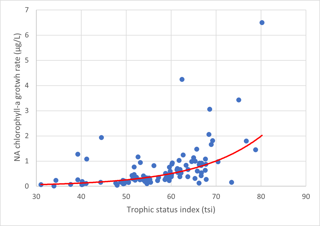
Figure 3a: The relationship between trophic states index (tsi) and chlorophyll-a growth rate in North America. Each dot represents a study lake. There are 101 samples in total. The trendline is shown in red and the type is exponential.
|
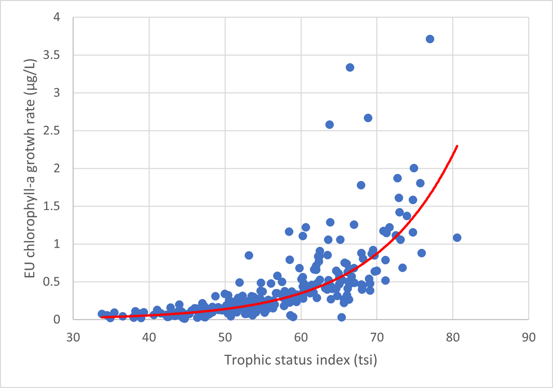
Figure 3b: The relationship between trophic states index (tsi) and chlorophyll-a growth rate in Europe. Each dot represents a study lake. There are 101 samples in total. The trendline is shown in red and the type is exponential.
|
The Figure 4 shows the result of principle component analysis (PCA). This graph can give a brief understanding about the relationships of these factors. The Proportion of Variance for PC1=40.08%, PC2=29.5%, which means 40.08% samples can be explained by first principal component and 29.5% samples can be explained by second principal component. So 59.58% which is the most of research samples can be explained by PC1 and PC2. The dots' color represents the trophic status of the sample lakes. This figure shows that the rate of increase in chlorophyll-a concentration (chla_rate), maximum chlorophyll-a concentration reached (max_chla), accumulated chlorophyll-a during the growth period (acc_chla) are highly positively related. With the positive direction of these few arrows, the color of the points is more red. This shows that they are also positively correlated with the TSI of the lake.
By observing other PCA vectors, Chlorophyll-a variables are positively affected by summer heat-moisture index (SHM), mean warmest month temperature (°C) (MWMT) and temperature average during the summer (Tave_sm). But the chlorophyll-a variables are negatively affected by precipitation during summer, spring and winter, both mean annual precipitation (MAP) and May to September precipitation (MSP), and annual heat-moisture index (AHM). And other factors which the vectors have nearly right angles may not affect Chlorophyll-a variables significantly.
By observing other PCA vectors, Chlorophyll-a variables are positively affected by summer heat-moisture index (SHM), mean warmest month temperature (°C) (MWMT) and temperature average during the summer (Tave_sm). But the chlorophyll-a variables are negatively affected by precipitation during summer, spring and winter, both mean annual precipitation (MAP) and May to September precipitation (MSP), and annual heat-moisture index (AHM). And other factors which the vectors have nearly right angles may not affect Chlorophyll-a variables significantly.
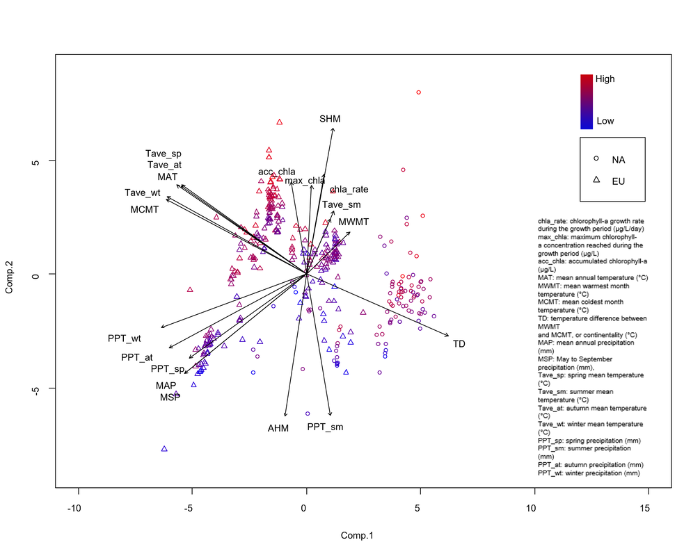
Figure 4: Principle component analysis of climate facotors and chlorophyll-a growth indicators. The different colors represent the trophic status of the lakes and the two shapes represent North America and Europe. Proportion of Variance for PC1=40.08%, PC2=29.5%.
R script
Figure 5a and 5b below shows the growth window period between lakes with different trophic status in North America and Europe. There is no apparent difference between them which proves the growth days may not affect the maximum chlorophyll-a concentration reached (max_chla) and accumulated chlorophyll-a during the growth period (acc_chla) significantly. However, the boxplots in Europe shows that the growth window length is relatively more close within and between trophic status.
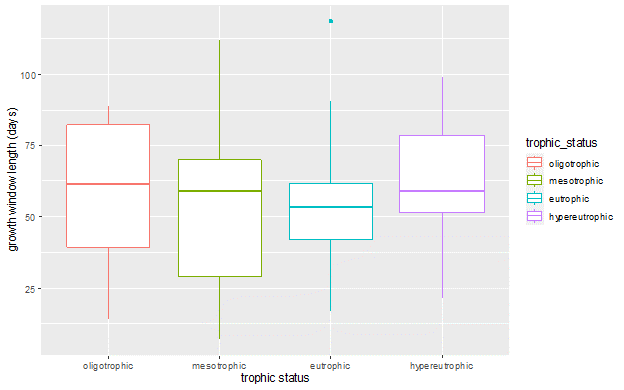
Figure 5a: The box plot for growth window period for lakes with different trophic status in North America. The colors show the different trophic status and listed on right. The dots represent the outliners and the top and bottom of straight lines show upper and lower limit. The horizontal thick line shows the median of the data. There are 101 samples in this graph.
|
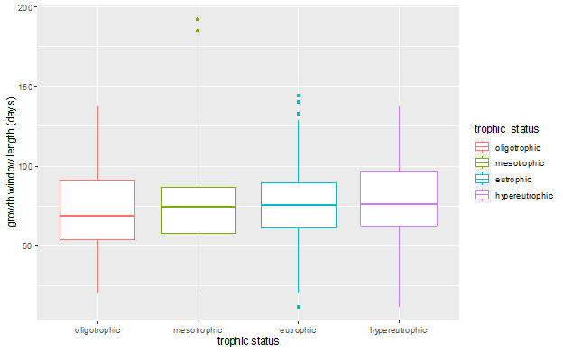
Figure 5b: The box plot for growth window period for lakes with different trophic status in Europe. The colors show the different trophic status and listed on right. The dots represent the outliners and the top and bottom of straight lines show upper and lower limit. The horizontal thick line shows the median of the data. There are 253 samples in this graph.
|
Sample R script
The combination of graphs below is the great scatterplot matrix by using ggpairs function. This matrix can give us an overview of the overall distribution of the data and the difference between different trophic statuses under different climatic conditions. Each dot on the lower left represents a sample of a lake. It shows the dot plot for each two variables. The diagonal shows the distribution of the four trophic statuses. The middle is high and the sides are low, indicating that most of the data is in the middle of the y-axis. The uneven distribution of left and right means that the distribution of data is not concentrated, which is shown in most of them. Due to more lakes are in eutrificatic status, there are more blue dots than other colors. This will also affect the total correlation coefficient which labelled in black color. The total correlation coefficient may be more close to the eutrophic samples. By observing and comparing different correlation coefficients, chlorophyll-a concentration (chla_rate), maximum concentration (max_chla) have different responses to changes in climate conditions under different trophic status. The explore and understanding of these difference is focused in this research. The more detailed trends and differences will be covered in results part.
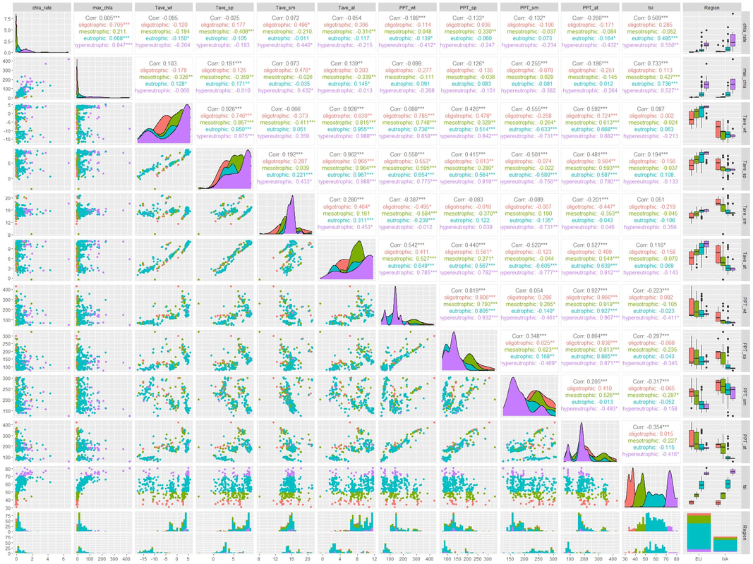
Figure 5: The ggpairs for indicators of chlorophyll-a concentration in lakes, with average temperature and precipitation from spring to winter. The sample number is 345 in each graph.
R script
